
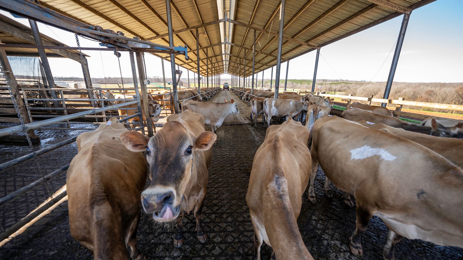
Spatial representativeness is broader than “distributing sensors evenly”
Drawing a grid on a barn plan and installing sensors at equal intervals can appear to cover the space fairly. In methane-emission measurement, however, the important issue is not dividing the floor area evenly. What matters is how well the result captures where methane is generated, which airflows carry it, and which boundaries it crosses when leaving.
For example, animals may congregate at feeding areas, while a manure pit is a separate source. If most of the air in a mechanically ventilated barn passes through a particular fan, that fan contributes more than a window with little flow. Openings in a naturally ventilated barn can switch between inlet and outlet roles with the wind. Under these conditions, evenly spaced sensors look orderly but create an uneven sample of emitted mass.
The U.S. EPA’s guidance on sampling designs for environmental data treats representativeness as a matter of study objectives and sampling design. It explains that even the highest-quality analysis cannot compensate for an unrepresentative sample. The same principle applies in barns.
Step 1: Define the measurement objective and spatial boundary first
Before selecting locations, determine which question the result must answer. The representative space differs depending on whether the objective is to find worker-exposure hazards, observe local concentration for ventilation control, calculate kg CH₄/h for one barn, or compare changes in enteric fermentation in a herd receiving low-methane feed.
For a safety objective, the worker’s breathing zone, manure-pit openings, ventilation dead zones, and worst-case conditions matter. For total emissions, the concentrations of incoming and outgoing air and the flow rate of each stream must be captured. A feed trial must be able to separate the air of the treatment herd from that of an untreated herd and from manure emissions. If one arrangement is used for multiple purposes, its suitability for each purpose must be validated separately.
A boundary drawing should show more than the barn walls. Mark animal areas; feeding, watering, and holding areas; manure pits and scraper routes; fans and air inlets; doors, windows, and ridge openings; adjacent barns and storage tanks; obstacles; and locations where sensor power and communications are available. Do not change the boundary for the convenience of sensor installation; choose a sampling method suited to the boundary that must be measured.
Step 2: Stratify the space by sources and airflow
Stratification divides a barn into areas with different characteristics. Overlaying the following four maps can produce practical strata.
Source map: mark where methane is generated, including animal density and residence time, feeding, manure accumulation and agitation, and storage facilities.
Airflow map: mark fan stages, air inlets, prevailing wind directions, temperature differences, obstructions, and short-circuit airflow.
Operations map: mark states that alter spatial distributions, such as open doors, movement for milking, cleaning, shipment, and minimum and maximum ventilation.
Interference map: mark adjacent barns, manure facilities and fuel sources, locations where exhaust re-enters, and candidate points for measuring the outdoor background.
Strata do not have to be the same size. If one fan group handles a large airflow, it can be treated as a separate stratum; a sidewall with frequent flow reversals can be managed as a bidirectional-flow stratum. Concentration trends at animal height and a cross-sectional average at an outlet serve different roles and should not be grouped in the same sensor set.
When creating strata, consider in advance which weights will be used in the calculation. The required measurement points become clear only after deciding whether the result is an area average, an animal-count-weighted average, or an airflow-weighted average. Total emissions generally require consideration of airflow and concentration together. A spatial mean concentration alone cannot distinguish the contribution of a high-flow, low-concentration area from that of a low-flow, high-concentration area.
Step 3: Conduct preliminary mapping before fixed installation
Do not determine actual flow from drawings and fluid simulations alone. Before installation, conduct a preliminary survey using mobile sensors, multipoint sampling lines, smoke or a safe tracer method, and air-speed and wind-direction instruments. The purpose is not to find “the highest point,” but to identify spatial variation and emission paths under each operating state.
The preliminary survey should include minimum, normal, and maximum ventilation and representative natural-wind directions. Examine events such as before and after feeding, animal movement, manure removal, and open doors separately. Do not record only methane concentration at each point; synchronize it with outdoor-air conditions, temperature and humidity, wind speed and direction, fan operation, opening status, and time.
When a sampling line switches sequentially among multiple points, transport time and sensor response time must be considered. Long tubing can delay the signal or condense moisture, and air from the previous point can remain just after a switch. Establish a stabilization time for each point and test line leakage and adsorption. Otherwise, genuine spatial differences will be confused with carryover in the sampling system.
Use the preliminary data to calculate correlations among points, differences in means, quantiles, and variation by operating state. Reduce nearby points that provide almost identical information and retain those that capture changes in direction or large concentration and airflow gradients. The purpose is not to minimize the number of sensors, but to reduce information loss with the limited number available.
Step 4: Arrange sensors for the ventilation type
In a mechanically ventilated barn, inlet and outlet paths are relatively clear, but do not assume that one point in front of a fan represents the entire cross-section. Use concentration traverses around the fan to examine the cross-sectional distribution and, if necessary, combine multipoint samples or apply airflow weighting to multiple points. The actual airflow of each fan requires field verification because it is affected by installed condition, static pressure, dust, shutters, and operating stage rather than determined solely by its nameplate value.
If not every fan operates continuously, the representative sensors and weights must change with the active fan group. Do not treat a stopped fan’s operating time as 0 airflow while applying the concentration in front of that fan to other fans. Measure a representative outdoor background for inlet concentration, avoiding points affected by exhaust recirculation or adjacent sources; if necessary, use multiple upwind points.
Naturally ventilated barns are more difficult. The direction and speed of flow through sidewalls, doors, and the ridge change with wind and temperature differences, and inflow and outflow can occur simultaneously within one opening. Fixed labels such as “inlet sensor” and “outlet sensor” are insufficient. Combine bidirectional air-speed and pressure information, multipoint concentrations, and weather data, then classify data by flow state.
Tracer-gas ratio or CO₂-balance methods can be considered for natural ventilation. A tracer gas must mix sufficiently with methane sources in space, and its release location and rate matter. A CO₂ balance depends on estimates of animal heat production and CO₂ generation, herd size, activity, and other CO₂ sources. Downwind concentration and a dispersion model can examine a farm-scale boundary, but require atmospheric stability, wind-field information, background data, and separation from adjacent sources. When methods are combined, verify that their boundaries are the same.
Step 5: Define aggregation rules and valid conditions together with the arrangement
Spatial representativeness does not end at sensor placement. How the values from multiple points are combined into one result is part of the arrangement design. A basic approach for total emissions is to calculate and sum airflow × concentration increase for each emission path. A simple average requires evidence that each point represents the same airflow and area.
Define valid conditions in advance as well. Document how to handle periods when wind speed is too low to determine flow direction, fan information is missing, the background sensor enters an exhaust plume, a sampling line is stabilizing after switching, or calibration has failed. Changing these conditions arbitrarily after seeing the result creates selection bias.
Manage the representative area and airflow for each point, state-specific weights, and exclusion rules in code and metadata. Distinguish a new arrangement version when the barn structure or fans change. Moving a sensor is not merely a maintenance record; it is an event that changes the measurement definition of the time series, so a period of parallel measurement before and after the move is advisable.
Step 6: Validate and revalidate representativeness in the field
The first validation compares fixed-sensor results with mobile multipoint mapping or a cross-sectionally integrated sample. Examine bias during minimum and maximum ventilation and major wind directions, not just normal conditions. An omission-sensitivity analysis that examines how much the overall estimate changes when selected points are removed is also useful. If removing one point changes the result substantially, the network depends excessively on that point.
The second validation compares the result with an independent method. Over a limited period, it can be compared with a tracer-gas method, CO₂ balance, respiration-chamber or head-chamber data, or downwind inverse modeling. Different methods have different boundaries and temporal resolutions, so their values need not be identical. Examine whether the difference lies within the expected range and whether its direction changes with operating state.
The third is a sensor-swap test. When Locations A and B have different values, swap the instruments and see whether the difference persists. If the difference follows the location, it is a spatial effect; if it follows the instrument, it is more likely a difference in calibration or response. Periodic collocation and standard-gas checks prevent sensor-to-sensor differences from being mistaken for spatial variation.
Revalidation should be triggered not only by calendar intervals but also by change events. Update the representativeness map after replacing a fan, installing a partition, changing stocking density, changing manure practices, relocating a sensor, or switching seasonal ventilation. Do not treat a fixed arrangement as a permanent answer.
Determine sensor count from variability and decision risk
It is difficult to provide one formulaic sensor count for every barn. A small mechanically ventilated building with little spatial variation and controlled emission paths requires a different design from a naturally ventilated cattle barn with large openings and multidirectional flows. Even in the same barn, the allowable uncertainty can differ between trend monitoring and verification of reductions for crediting.
Determine the count using the spatial variance and inter-point correlations in preliminary data, the required total uncertainty, and the cost of a wrong decision. Examine how much adding one sensor reduces uncertainty in the final emissions result. If the reduction is negligible, it may duplicate the same area; if it is substantial only under a particular state, a mobile supplementary measurement for that state may be more efficient.
The cost of spatial representativeness includes not only sensor prices, but also calibration, standard gas, line maintenance, communications, recovery of missing data, and staff time for data review. A small network that is validated and maintained is better than a large network that cannot be operated.
Implementation checklist
Have the measurement objectives for safety, operations, total emissions, and feed effects each been defined separately?
Have the spatial boundaries of barns, herds, manure facilities, and adjacent sources been marked on a drawing?
Were source, airflow, operations, and interference maps overlaid to stratify representative areas?
Was pre-installation mapping conducted under minimum, normal, and maximum ventilation and major wind directions?
Were the concentration and actual airflow distributions across outlet cross-sections validated?
Does the design address flow reversals and bidirectional flow at naturally ventilated openings?
Was it checked whether the background sensor is affected by exhaust recirculation and adjacent plumes?
Are the representative airflow and area for each sensor and the aggregation weights documented?
Were location effects validated through sensor swaps, collocation, and comparison with an independent method?
Is there a rule that triggers revalidation when the structure, fans, herd, or season changes?
Conclusion: a good arrangement is completed by evidence, not a drawing
Spatial representativeness is not a matter of placing many sensors symmetrically or attractively. It requires understanding methane sources and airflow, defining a boundary appropriate to the purpose, and connecting each point to the airflow and space for which it is responsible. Pre-installation mapping, stratification by state, airflow-weighted aggregation, and field validation provide the evidence for that connection.
A barn is a living operating environment. When seasons, wind, stocking density, and equipment change, there is no guarantee that yesterday’s representative point remains representative today. The sensor layout must therefore be managed as a versioned measurement model rather than a one-time installation document. Only an observation network designed this way can turn local concentration readings into defensible data for assessing barn emissions and reductions.
Sources
Guidance for Choosing a Sampling Design for Environmental Data Collection, EPA QA/G-5S — U.S. Environmental Protection Agency
EPA Quality Assurance Handbook for Air Pollution Measurement Systems, Volume II — U.S. Environmental Protection Agency
FAO: Methane emissions in livestock and rice systems — Food and Agriculture Organization of the United Nations
Methane emission from naturally ventilated livestock buildings can be determined from gas concentration measurements — U.S. EPA HERO literature record
Methods for measuring gas emissions from naturally ventilated livestock buildings — U.S. EPA HERO literature record
Heat balance and tracer gas technique for airflow rates measurement in naturally ventilated livestock buildings — U.S. EPA HERO literature record