
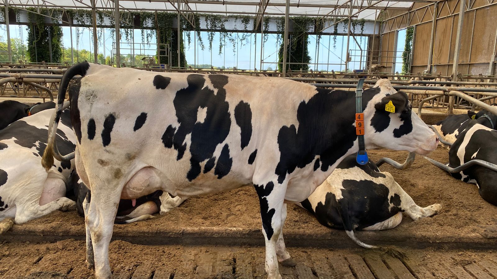
If methane concentrations fall in the week after low-methane feed is introduced, can we say that the feed caused the reduction? The earlier event and the later outcome may appear connected, but timing alone does not establish causality. During the same period, temperatures may have fallen, ventilation settings may have changed, the herd size may have decreased, or feed intake and productivity may have shifted. Sensor calibration or measurement locations may also have changed.
Establishing causality means using study design to estimate the counterfactual: “What would have happened to methane in the same animals or on the same farm if the feed had not been introduced?” Because the same animal cannot be in treated and untreated states at the same time, researchers use control groups, random assignment, crossover designs, repeated measurements, and statistical models.
Why before-and-after comparisons often go wrong
The simplest design compares the average before introduction with the average afterward. This is convenient in farm operations, but it confounds seasonal trends with the feed effect. For example, if the baseline period falls in midsummer and the intervention period in early autumn, heat stress, feed intake, and ventilation will all differ. Even if methane falls by 10%, it is difficult to isolate how much of that change came from the feed.
Regression to the mean also requires attention. If a week with unusually high methane values is selected as the baseline, subsequent values may return to their usual level even without any intervention. Conversely, sensor drift that coincides with the introduction date can create a false effect. The visual observation that “the introduction date matches the drop in the graph” can support a hypothesis, but it cannot establish the size of the effect.
Another source of confusion is the choice of metric. g CH₄/day, g CH₄/kg dry matter intake, g CH₄/kg milk, and the average ppm in a barn answer different questions. If the feed lowers total methane while also reducing intake or output, the environmental and production implications may differ. The FAO LEAP guidelines for feed additives recommend comparing environmental performance across the supply chain, including additive production and use, with a consistent life-cycle assessment method. A decrease in a single enteric-fermentation metric does not automatically establish overall environmental performance.
Causal designs that can be used in the field
The easiest design to understand uses a concurrent control group. Similar animals are randomly assigned to treatment and control groups and observed over the same period under the same barn operating conditions. Random assignment reduces the chance that both known factors and unanticipated animal-level differences will be concentrated in one group. If the number of animals is small, blocks can first be formed using key characteristics such as weight, parity, days in milk, and output, followed by assignment within each block.
A crossover design can make each animal its own control. One group receives the control feed followed by the test feed, while the other group receives them in the reverse order. This can reduce between-animal differences, but the design must account for carryover effects in which the previous treatment continues to affect the next period. Provide an adequate adaptation period and, where necessary, a washout period, and include period and sequence effects in the analysis. Because feed can take time to change the rumen environment, conclusions should not be based only on a few days immediately after introduction.
When treatment is applied at the farm level, consider a cluster design that assigns multiple farms to treatment and comparison groups. Treating the many sensor observations from one farm as hundreds of independent samples creates pseudoreplication and inflates the sample size. If the intervention is applied to the farm, the experimental unit may be the farm, with animal and time measurements nested within it.
In commercial settings where randomization is impossible, quasi-experimental designs such as difference-in-differences and interrupted time series can be used. These methods still require assumptions—for example, that comparison farms followed the same external trends or that no other intervention occurred at the same time. The assumptions should be assessed in advance using graphs and operating records, and the limitations must be disclosed.
The measurement plan must match the experimental design
ICAR guidance explains that the suitability of respiration chambers, SF₆, GreenFeed, sniffers, portable accumulation chambers, and proxy indicators differs according to the required outcome and field conditions. The same equipment is not always best for a trial that seeks absolute emissions and one that seeks to rank individual animals. Do not select equipment first and then force the question to fit; define the primary (1st) endpoint and required accuracy first.
Measurements should not be concentrated only in the period immediately after feeding on a particular day. Methane emissions from ruminants follow feeding and diurnal patterns. ICAR’s GreenFeed procedure sets out operating principles for spreading visit measurements across the day and obtaining background concentrations and quantitative flow. Whatever the method, measurement opportunities, access to equipment, and missing-data rules must be kept the same for treatment and control groups.
Feed exposure must also be measured. Including an additive in the formulation is not the same as each animal actually consuming the target dose. Record the batch number, formulation concentration, amount offered, residual amount, individual access records, dates of interruption, and adverse reactions. Selecting only animals that complied with the feeding plan after seeing the data can create selection bias by removing animals with low adherence, so the primary analysis population should be defined in advance.
Criteria to agree before analysis
Document the primary (1st) outcome, comparison periods, exclusion criteria, minimum data availability, statistical model, and significance level before examining the data. Where possible, determine the sample size through a power calculation that considers not only the expected effect but also variation between animals and days and measurement error. A nonsignificant result in a small sample does not mean “there is no effect,” and even a significant result may be imprecise if the effect size and confidence interval are wide.
In addition to treatment, the analysis may include prespecified covariates such as baseline values, parity, stage of lactation, dry matter intake, production, weather, and ventilation. However, automatically controlling for a variable that changed as a consequence of treatment can remove part of the genuine effect. It is useful to map the causal pathway first and distinguish confounders from mediators.
After obtaining a favorable result for one metric and period, repeatedly changing the subgroups and time periods to select only favorable results magnifies the multiple-testing problem. Label exploratory analyses as exploratory and distinguish them from confirmatory trials. Reproducibility of the effect should also be assessed in other seasons, on other farms, with other feed batches, and through independent analysis.
Implementation checklist
Use a concurrent control group or a valid quasi-experimental comparison to represent “what would have happened without the feed.”
Specify whether the experimental unit is the animal, barn, or farm, and avoid pseudoreplication.
Prespecify random assignment, blocking, crossover sequence, and adaptation and washout periods.
Register the primary (1st) endpoint and unit, measurement method, sample size, and exclusion and missing-data rules.
Record actual intake and batch details, feeding interruptions, and productivity and health indicators together.
Apply the same measurement schedule and quality standards to treatment and control groups.
Report the effect size, confidence interval, data availability, and sensitivity analyses together.
Distinguish reductions in enteric fermentation from product-level environmental performance, safety, and productivity.
Conclusion
The causal effect of low-methane feed does not emerge from a single before-and-after graph. A comparable control condition must be created, animal-level differences separated from changes over time, actual intake and measurement quality confirmed, and analysis rules set before the results are known. Field trials are more complex than laboratory studies, but credibility begins by incorporating that complexity into the design and analysis rather than erasing it from the records. Only results that pass through this process can move beyond “they changed together” toward the claim that “the feed contributed to the change.”